Hey guys. For the second time for me now this time has come. I'm in the finish line of GSoC. For the second time I was working on LabPlot with my awesome mentors, Alexander and Stefan. We've been working on this project together, without their help we wouldn't be here. As you could read in my previous post, we were quite close to the main aim of the project already then but we were still missing a few things like reading from sockets. Those problems are solved since then, but like in real life there are always new ones. Our main focus in the continuation of this part of LabPlot is the performance improvement. I have since the previous post fixed the reading from local, tcp, udp sockets. We have fixed a couple of bugs, implemented preview for sockets, did some performance improvements on plotting. In the future we are considering the following steps according performance: parallelization of the plotting, use different threads for data read to avoid UI blocking, algorithmic optimizations. Another thing we need to finish is the reading from serial port, we had a hard time with it till now, but we'll surely find a way to fix it.
I made a demo video in which I use LabPlot as a monitoring tool. Here I'm sending data though a TCP socket using a python script. I'm sending a few values, like cpu usages, memory usage, swap memory usage, disk usage. You can see the live data read and plotted in LabPlot. You can also see that we have fixed/implemented the data ranging, only a number of data points are plotted if you look closely in my video.
You can watch the demo video here:
Here is how the preview for TCP sockets looks like:
Preview for TCP socket
It's been again a great experience to learn new things, techniques during this GSoC. You can read "but not in the end" in the title, this means that the end of this program shouldn't mean that we quit contributing to open source software. I am sure that all of us had great moments of success during GSoC and I think as we use a lot of software for free we should give something back to the open source community. If it would be possible I would apply again to be a GSoC student again next year or anytime.
Thanks for the moments, thanks for the read and huge thanks again to my mentors, Alexander Semke and Stefan Gerlach.
In the future I'll be posting here stuff we work on in Labplot, so keep an eye here :)
Hey guys. It's been a while since my last post here, but we did a good job meanwhile. Beside implementing the features I have described in my previous post I have implemented some other useful features/additional options. Let's see what we have here.
First of all I'll just list the options that are implemented already and in the end I'll talk a bit about the next steps.
Source type
File or named pipe
Network TCP socket
Network UDP socket
Local socket
Serial port
Reading type
Continuously fixed
From end
Till the end
Update type
Periodically
On new data
Keep last N values
Update now
Pause/Continue
Update interval
Sample rate
As I told you, for "Periodically" update type the user has to provide a value in milliseconds (planning to extend this to other interval types such as minutes, formatted time values..). For "Continuously fixed" and "From end" reading types the user has to provide a value which is the sample rate. On every update we'll read sample rate number of samples if they're available.
The option that I had no words about in my previous post is the "Reading type" one. Let's think a bit, if we have a device that sends lots of data then we may want to check only a piece from the end of the data. For this we have the "From end" reading type. It's possible that we want to observe continuously this new data, but read just some samples at a time. For this we have the "Continuously fixed" reading type. Also it's possible that we need all of the new data every time we update. In this case we have a third reading type, this is the "Till the end" one. For the "Continuously fixed" and "From end" the user must provide a value (sample rate) to tell LabPlot how many lines he/she wants to read on every update. No worries if the user enters a larger number than the actual new lines, we'll read just as much as we have in that case.
Using our new LiveDataDock we allow users to change almost every option while doing the actual reading. Only the "Keep last N values" cannot be changed, because if we use that we want to have a fixed size that's not changing.
The new reading type option in "action":
Reading types
After creating the FileDataSource we get the newly implemented LiveDataDock. For "Till the end" as I said we don't need sample rate, so in that case LiveDataDock looks like this:
Till the end reading type selected
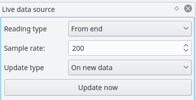
But if the "From end" reading type is selected then the Sample rate line edit shows up:
From end reading type
In the other hand if the user wants to read the new data only if there is actually new data then this can be done as explained in my previous post, using the "On new data" update type:
From end with On new data
For almost every of the newly implemented features I have an example video which was made right after I got it working.
In this video I'm presenting the use of the "Update interval" option.
This video is about changing the sample rate and pausing/continuing the reading.
The "Update now" button is presented in the video above.
This one demonstrates the "Keep last N values" option in action.
As you can see I have spent lots of time in these demo videos with the plot setup. We knew we need to speed up this procedure, so one of my mentors (Alexander Semke) implemented the PlotDataDialog for FileDataSources and so in just 1-2 clicks we can get our data plotted nicely.
Then I came up with an idea which I thought we need for live data, but as we talked with Alexander I realized that this feature is useful for static data too. This feature is the data ranging, which consists of setting the plot's X min and max values to a calculated one. We get this value after providing the number of samples we want to see plotted from the end or the beginning of our FileDataSource. This feature is currently in development, but it will be soon working. This new feature is added to the CartesianPlotDock:
CartesianPlot data range
The "Free ranges" data range will be the same as it was available in LabPlot before. For live data sources the "Show last" option makes more sense, but in case of fixed sized FileDataSources even the "Show first" option can be useful. These options take a value which means the number of samples to be plotted. Using "Show last" we can watch the latest N new samples plotted. As I was thinking about this feature I "hacked" a fast prototype to demonstrate my idea about the "Show last" option to Alexander, you can check it here:
Here I'm using the PlotDataDialog for FileDataSources, you can see the difference I guess :).
About the source types: we need to learn a bit about the data extraction from sockets and every source type should be working just fine.
About the next steps, there can be lots always. The first steps are to fix the data extraction from sockets. After this we will be working on optimizing the data plotting which wasn't really designed for growing/frequently changing data, but we'll try our best to make LabPlot better and faster :)
This was for now folks, thanks for your attention, check out LabPlot! See you! :)
As I told you guys in my previous post, I'm here now to show you some new, cool stuff about LabPlot. First let me introduce you the synopsis of my project's proposal:
"Currently, the visualization and analysis of data is only possible on static data that was imported into or generated in one of LabPlot's data containers. The goal of the project is to add support for streaming data. At the moment LabPlot has no support for this kind of data processing even though it is very important for this feature to be available in a scientific data plotting software."
As you can see one of the main tasks here is to be able to handle changing, streaming data. Somebody may plug in their physical device and then watch as their datas are being plotted. For this to work nicely and user friendly, we collected a handful of options to control this kind of data source. The first thing you want to do is to create a new FileDataSource, you can do that this way:
FileDataSource creation
After this you get this nice looking dialog with the new options, controls. We decided to support more types of live data sources, as you can see in the picture below.
FileDataSources options
For "File or named pipe" source type we have the following options:
File or named pipe options
This kind of source consists of reading from a local ascii or binary file or a named pipe. A named pipe is a bit more than a traditional pipe because it has a name and unlike the traditional one it can last till the system is up. In Unix systems one has to explicitly create a named pipe using mkfifo or mknod. After creation one process can write to it and one can read from it by name. Also for "Local socket" live data source type we have the same options, but this consist of reading from a local socket using QLocalSocket. To work with QLocalSocket we just need the name of the server the socket is connected to.
The next type of live data source is the Network socket one. The following options we have right now to configure this kind of live data source:
Network socket options
A network socket is an endpoint for sending/receiving data in a computer network. In our situation we want to read from it. To access a socket we must have the socket host's address and port number.
The last type of live data source for now is the Serial port one. In the following picture you can see the options for this kind of data source:
Serial port options
This kind of live data source consist of reading from a port to which a physical device is connected. We just have to select the port our device is connected to, set the baud rate and voilá, it should work nicely soon. We use QSerialPort to access, work with serial ports. Using QSerialPortInfo class we can have informations easily about the available ports on our system. Also the supported baud rates can be acquired using QSerialPortInfo.
These options are necessary to set up the wanted kind of live data source. Beside this we must have some control above this kind of data source, right now we have the following options to control the update a FileDataSource:
Update options
Here you can see that we have two types of updates. The "Time interval" one will update the curves on a specified time interval (every second, every five seconds or so) which is a value in milliseconds. The "New data" update type will update the curves only when there's new data available. In the "Update frequency" we set the interval between the updates when using "Time interval" update type. The "Keep last N values" will control how much of the data we want to update. For this kind of data source one usually want to observe how the data is changing, to take a snapshot of their data.
Another thing we might want is to have control over this kind of data source even after creation. For this we'll have a dock widget, it's not yet used, but currently it looks like this in Creator:
FileDataSource dock widget
With these options we will be able to modify the number of values we want to keep on every update, the time between updates. If the user uses a long interval between the updates then a functionality like the "Update now" button will provide it's very useful because there might be moments we didn't think we'd need to check the actual state of our data. Also the pausing and stopping the updates/data reading helps in the control of this kind of data source.
I have created a demo video which shows the creation of a FileDataSource, setting the X and Y axis data of some xy curves. Then a python script writes Brownians motion data to a file on which the FileDataSource was created. We can see there the curves being updated on new data:
An issue you can see here is that I have to set for every curve separately the X and Y value columns. We will use the PlotDataDialog which is used for plotting spreadsheet columns to solve this issue. PlotDataDialog is a very user friendly dialog which can be accessed from the spreadsheet's context menu. In this dialog we can select the X data and Y data for any curves we might want to plot from spreadsheet column data. This is the PlotDataDialog:
PlotDataDialog
This is for now, hope you guys enjoyed it! The next step is to implement all the logic behind these options and make them do their job. A greater step after implementing the options will be to optimize our code on larger amount of data. Thanks to my mentors, Alexander and Stefan for their great help. Every time I am unsure on something they take their time to talk about it so together we can make LabPlot even cooler than it is right now :).
See you guys soon again! Have fun on your GSoC project!
Hi folks, it's been a while since my last post here. I had a hard time to start on GSoC but now that I have successfully graduated from the university (Computer Science BSc) I have all my time for my project. While learning for the exams and preparing for my final exam I've been talking to my mentors often to share our ideas about the project. Thanks to the fact that I have already worked previously (and continously after GSoC) on LabPlot I can implement the needed features much easier and quicker now than last year :) Now that I have my own branch and a few new classes added I can continue the adventure with LabPlot! See you soon! :)
So we are here, GSoC 2016 is officially over, it's time for the final evaluations, so this will be a closing post for this GSoC. I've learned many things while I was working on my project and I'm really thankful to my mentors, Stefan and Alexander (not officially my mentor, but we talked many times and he helped me many times too). I'll be happy to help in integration of this project in the next release of LabPlot :)
Since my last post I've fixed some minor bugs, and implemented some new features too.
Let's say we want to add a new keyword to one of our FITS extension:
FITS header editor's new keyword adding dialog
And then we can add units to our keyword, which will appear in squared bracelets in the beginning of the comment:
Keyword unit adding dialog
I added some predefined units, such as meters, kilograms, seconds, parsec, solar mass, astronomical unit, kelvin, light year.
The newly added keyword unit
If a keyword has some kind of unit defined already, then the dialog will be shown with the unit of the keyword:
Saving keyword modifications
We have modified this value, the original is "lw", as you can see in the treeview.
The saved extension with the new keywords value
As you can see, after saving the modifications, and reopening the file, the name of the extension is modified.
Import a subset of data
Let's say we have this image, but we'd like to import just a portion of it.
We just have to set the start/end row/columns in the import dialog,
..and voilá
File info dialog improved for FITS files
Import FITS tables to matrices
If the selected table extension has numeric columns (at least one) then we can import those in matrices. (btw notice the nice icons in the treeview, thanks to Alexander for the idea)
As you can see, the second and third column contains only values, so after import our matrix:
I think this was it. I hope you enjoyed it too. I'm really happy that I was part of GSoC '16, it's one of my greatest experiences. I look forward on reading other GSoC students blogs and I wish good luck to everybody on the final evaluation! :)
I have implemented some features since my last post, soon I'll be polishing the features, searching for bugs. So, let's have a look at them:
Delete FITS extensions from files:
Context menu for deleting extensions
You just right-click on the extensions, and you can delete them, and after you save the file, reopen it, you can check the file again:
(I deleted the other extensions this time) And you can see that some extensions are removed from the file.
I've improved the export dialog for FITS files:
Now you can select whether you want to export your container to an image extension, or a table. If the spreadsheet contains non-numeric columns, then exporting to a FITS image it's not possible:
You can check the "Columns comments as units" checkbox if you'd like to export the column's comments as FITS table units, check comment:
And here you can see it as the unit of the column in the FITS table:
Other important it's that when you import tables to spreadsheets, then columnmodes are set properly, for example text/numeric columns:
To prove that:
In short, "A1" stands for a column which contains strings, with length of 1.
That's for now, I'd be happy if you could test the features/give feedback. See you soon.:)
There are some new features that I've implemented since my last posts, let's see them!
FITS tables can be imported to spreadsheets now. Let's see how it works:
FITS table imported to a spreadsheet
As before, I compare my results with the results of FV (FITS Verify). I set the column comments to the units defined for the columns in the FITS if they're available.
You can now export your matrices to FITS images! If the file exists, it just appends a new image extension, if not, it creates a new FITS file, check out the header of an exported matrix, and the tree of the file:
Header keywords of the exported matrix
You can export your spreadsheets to FITS tables too!
Currently the export dialog for FITS files
And then you can check out your file's header:
Header of the exported FITS file
Great, isn't is?! If the file didn't exist yet, it creates one with an empty primary array, and appends an ASCII table. It still needs more improvements of course.
And then let's import back our exported spreadsheet:
The exported spreadsheet imported
There are still plenty of things to fix, and others to implement of course :)